To observe the inside of an object, we require high-energy photons such as X-rays and gamma radiation. Typically, imaging using X-rays or gamma radiation involves positioning the target between the radiation source and the detector. However, in many cases, it is not feasible to place the detector in the opposite direction to the source. Examples of such situations include detecting or imaging buried objects such as landmines, the inner side of pipes or walls, and others. The Compton Camera is a deviced developed by researchers in Bogotá and Darmstadt and lead by the Nuclear physics group of the Universidad Nacional de Colombia GFNUN, which uses backscattered gamma photons to produce images.

Device working principle

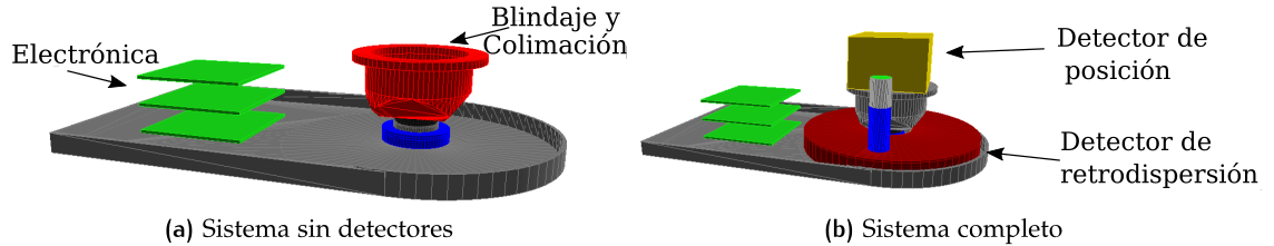
The GFNUN Compton Camera consists of an array of two detectors set up in a coincidence configuration. The backscattering detector is shaped like a hollow cylinder, with a lead shielding containing a ^22^Na radioactive source located within the hole. This detector is made of a CsI crystal coupled to two photomultipliers. The position detector, on the other hand, is a CsI crystal with a special photomultiplier that allows for the current generated to be divided into a 64x64 pixel grid. The working principle of the camera is the following:

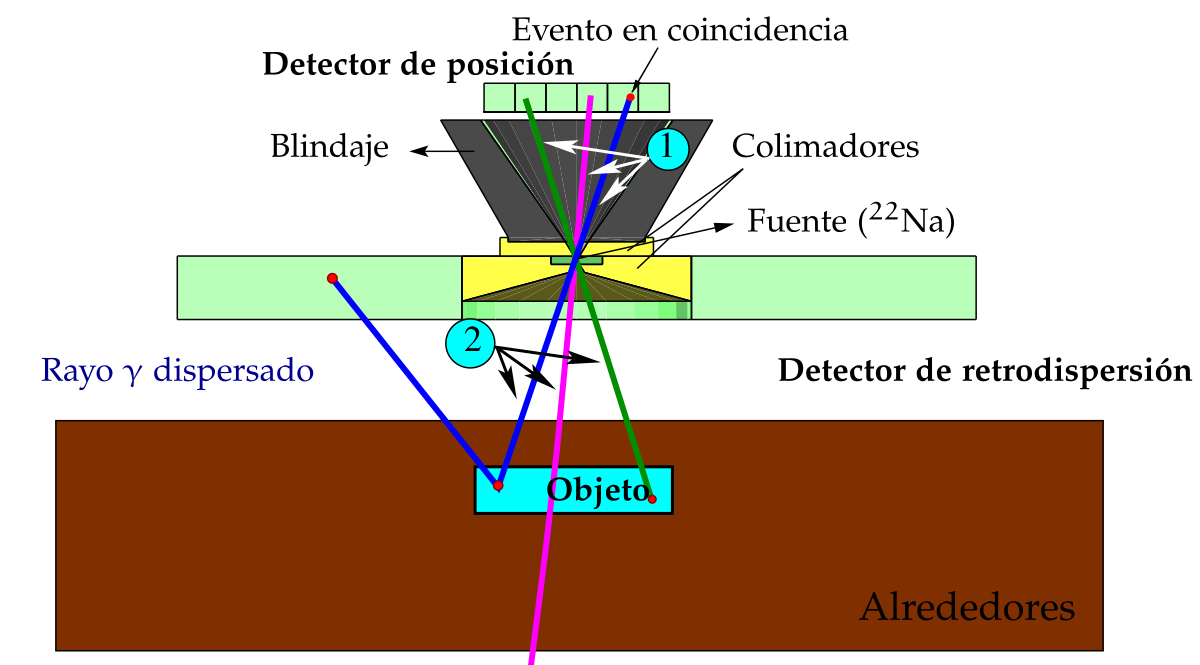
A beta decay occurs inside the source, producing an electron-positron pair that annihilates and creates a pair of 511 keV photons. These photons travel in opposite directions.
One photon travels towards the position detector while the other travels towards the sample.
The photon traveling towards the sample may undergo one or multiple backscattering events with the sample or its surroundings, eventually reaching the backscattering detector.
Once the backscattering detector registers the backscattered photon, the position detector saves the position (adding one count to the pixel) of the first photon that traveled towards it. A time window is fine-tuned to allow for “waiting for the signal”, and if no photons arrive at the backscattering detector, no pixels will be filled in the position detector.
This process is repeated for several photons. Due to the spatial distribution of the sample, differences in materials (primarily densities), and energies, an image is created as a result of the difference in the probability of the photons being scattered.

The single backscattering equation

A toy model can help provide an intuitive understanding of how the number of backscattered photons is influenced by the material and energy of the incident photon. This model assumes a uniform single-element material and perfectly collimated photons. Under these circumstances, the number of backscattered photons can be expressed as follows:

where $I_{0}$ is the incident intensity of photons, $B(E_{\gamma},x)$ is the buildup term, $\mu$ is the attenuation coefficient for the incident photons, $\mu(\theta)$ is the attenuation coefficient for the single backscattered photons (which, in general, depends on the energy), Z is the atomic number/effective number of the material, $n(x)$ is the number density (which depends on the molar density of the material), $d$ is the thickness of the dispersing material, and $\frac{\sigma_{k}}{d\Omega}$ is the Klein-Nishina differential cross section.

Assuming there are not multiple dispersion and the source is perfeclty collimated, then $B(E_{\gamma},x)=1$, and if the material is homegeneous the number density is independent on the position, we can summarize the equation for the backscattered photons as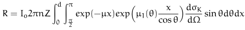

GEANT4 simulation

To improve the device design and enhance the quality of the images produced, we utilize Monte Carlo simulations. We use the widely-used toolkit, GEANT4, which is popular in the fields of particle and medical physics and can be used for most studies involving the passage of radiation through materials.

We tested various materials for the detectors, as well as different geometrical configurations, and a pure beta decay source. By running simulations with different parameters, we can evaluate how they affect the image quality and optimize the design of the device for improved performance.

Although the backscattering detector is used as time trigger, we can obtain from the simulation the energy spectra and compare it with the observed in the laboratory one.

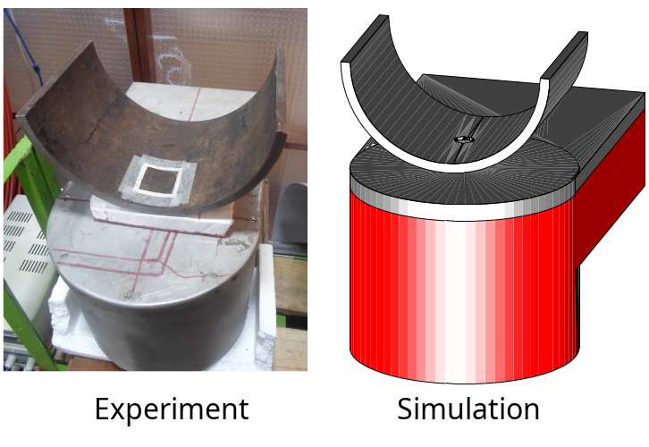
Case study I: Examining the inner region of a corroded tube

Corrosion and erosion can cause pipes in pipelines (such as those used for oil, gas, and water) to fracture. This process starts at the surface, but examining the inner surface of a pipeline can be challenging and may require breaking it. In this case study, we aim to demonstrate the capabilities of the Compton Camera for imaging a corroded tube from the inner side.

The image below shows the simulation and the experimental setup of the imaging system. Notice the defect of the tube is located in the innerside, and the camera is located in the opposite site.

Comparison of images of the defect inside a pipe, when using a visible camera we changed the direction where the camera is pointing, if the visible camera is located in the same direction than the gamma camera then the defect would not be observed. Recall that the Compton camera image is obtained using photons that were backsattered (this is not a transmition technique)

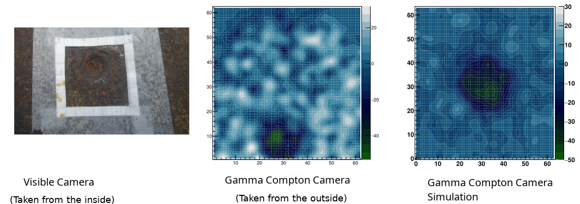
The experimental centering of the sample was innacurate that is why the circular region representing the defect is towards the bottom of the image.

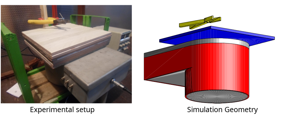
Case study II: localizing objects inside/behind a wall

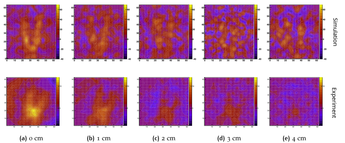
Another example where transmitted photons are not accessible and backscattering techniques are required is in the imaging of buried objects (such as landmines) or objects hidden behind thick surfaces like walls. In this study, we will investigate the capabilities of the Compton Camera to image one object (pliers) behind ceramics, and gradually increase the ceramic thickness until the object can no longer be distinguished. The figure below depicts the experimental setup, as well as the simulation geometry.

Below is presented the images obtained with the Compton camera and the simulated version of the same setup. It was obseved that for the current version of the camera we have a maximum depth of around 5 cm. However this is highly dependent on the involved materials.