Rho-statistics are the two-point correlation function (2PCF) of residual errors from the Point Spread Function (PSF) modeling. Stars are point sources, and the images we obtain from stars are actually a representation of the PSF. Therefore, we can use images of stars for modeling the PSF. The PSF has two main contributions: the optics of the telescope and the atmospheric smearing, and it is position and wavelength-dependent. The PSF needs to be interpolated to the galaxy’s position, and this interpolation might introduce errors given the variance of the PSF across the field of view. To study systematic biases that might arise from the interpolation scheme, a set of stars is left out from the PSF modeling. Then, by comparing the shape measurements of those reserved stars with the expected shape using the interpolation scheme, we can obtain residuals of the PSF that will help identify problematic sources, exposures, or regions where the PSF systematics exceed the requirements. Additionally, we can use these residuals as building blocks of PSF residual point correlation functions, which can be propagated in the likelihood analysis to study the consequences on final cosmological estimates.

PSF errors

Biases in weak gravitational lensing are studied using the linear approximation

\[\begin{equation} \hat{g_{i}}-g^{\rm{true}}_{i}=\mu_{i}g^{\rm{true}}_{i}+c_{i}+\rm{noise}, \label{eq:biasdef} \end{equation}\]

where the mutiplicative bias $\mu_{i}$ and the additive one $c_{i}$ are obtained using a linear regression for a population of galaxies. To see the effect of miss estimation of PSF, we can consider as an estimator the observerd ellipticity without the correction for the PSF, and make simulations of galaxies with different shear values and PSF. For avoiding other sources of biases and see just the PSF ones, we simulate only one galaxy with just a $e_{2}$ component, and sheared only in the first component direction, this garantees there is not shape noise.

PSF size errors

When changing only the size of the PSF and keeping it circular, we can observe a multiplicative bias contribution. As ilustrated in the animation below wehre as sheare estimator HSM is used.

PSF anisotropy errors

When changing the ellipticity of the PSF, we can observe an additive contribution to the bias, when there is change in the first component of the shear PSF ellipticity, and a subtle multiplicative bias when the PSF is aligned with the galaxy ellipticity as ilustrated below

In the Y3 analysis of DES the effects of PSF biases in comology goes like follows:

The multiplicative bias is treated as a nuisance parameter in the likelihood, there is one for each of the four tomographic bins, and the mean and prior range are determined using simulations.
The addive bias could be treated similarly, however his contribution can be neglected if we observe the PSF additive contamination in the 2PCF to be subdominant.

Rho statistics

We can write the additive systematics in the ellipticity estimator as $\begin{equation} e^{\textrm{gal}}=\gamma+\delta e^{\textrm{sys}}+\delta e^{\textrm{noise}}. \label{eq:observed} \end{equation}$ To get the PSF associated part of $\delta e^{\textrm{sys}}$, the parametrization

\[\begin{equation} \delta e^{\textrm{sys}}_{\textrm{PSF}}=\alpha e^{\textrm{p}}+\beta\left(e^{\textrm{*}}-e^{p}\right)+\eta\left(e^{*}\frac{T^{\textrm{*}}-T^{p}}{T^{\textrm{*}}}\right), \label{eq:new} \end{equation}\]

is proposed where field with the * symbol are measurements of the reserved stars not used during the PSF modelling, and the $p$ label are the PSF values interpolated at the position of those stars. The previous parametrization is justified when doing gaussian propagation of errors using unweighted moments. The first term correspond to the PSF leakage, second one is the error associated to PSF shape residuals $q=e^{*}-e^{\textrm{p}}$, and the third one to PSF size residuals $w = e^{*}\frac{T^{\textrm{*}}-T^{p}}{T^{\textrm{*}}}$, using that notation we can write

\[\begin{equation} \delta e^{\textrm{sys}}_{\textrm{PSF}}=\alpha e^{\textrm{p}}+\beta q+\eta w. \label{eq:simple} \end{equation}\]

Now, we want to determine the parameters $\alpha$, $\beta$ and $\eta$ fitting a model involving star-galaxy correlation. The 2PCF of each PSF systematic field with the galaxy shape estimator is

\[\begin{align} \left\langle e^{\textrm{gal}} e^{\textrm{p}} \right\rangle &= \left\langle \delta e^{\textrm{sys}}_{\textrm{PSF}} e^{p} \right\rangle+\left\langle \gamma \right\rangle \left\langle e^{p} \right\rangle \label{eq:firstsystemofeqrhosys1} \\ \left\langle e^{\textrm{gal}} q \right\rangle &= \left\langle \delta e^{\textrm{sys}}_{\textrm{PSF}} q\right\rangle +\left\langle \gamma \right\rangle \left\langle q \right\rangle \label{eq:firstsystemofeqrhosys2} \\ \left\langle e^{\textrm{gal}} w \right\rangle &= \left\langle \delta e^{\textrm{sys}}_{\textrm{PSF}} w\right\rangle +\left\langle \gamma \right\rangle \left\langle w \right\rangle \label{eq:firstsystemofeqrhosys3} . \end{align}\]

To symply calculation we can work with mean subtracted fields, we introduce the primed notation, $x'=x-\left\langle x \right\rangle$. Defining the Tau statistics as

\[\begin{equation} \tau_{0}=\left\langle e^{\textrm{gal}'}e^{p'}\right\rangle \quad , \quad \tau_{2}=\left\langle e^{\textrm{gal}'}q'\right\rangle \quad , \quad \tau_{5}= \left\langle e^{\textrm{gal}'}w'\right\rangle \end{equation}\]

and introducing the stars correlation, $\textbf{Rho-statics}$,

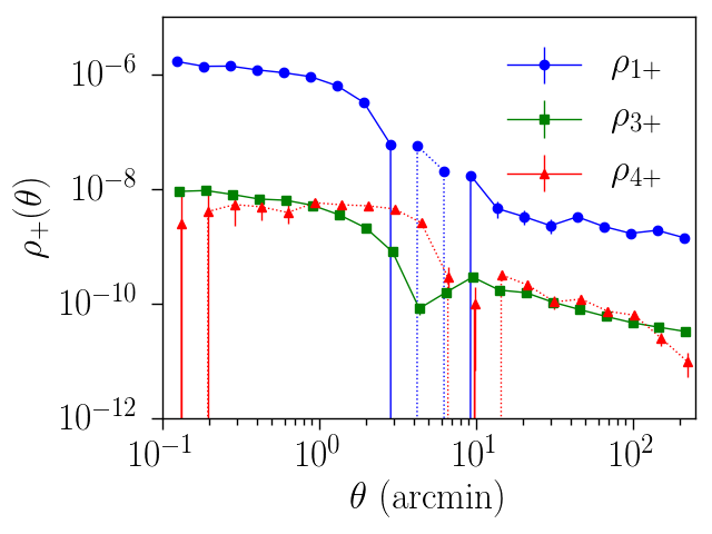
\[\begin{equation} \boxed{ \begin{aligned} \rho_{0}=\left\langle e^{p'}e^{p'} \right\rangle \quad , \quad \rho_{1}= \left\langle q'q' \right\rangle \quad , \quad \rho_{2}= \left\langle q'e^{p'} \right\rangle, \\ \rho_{3}= \left\langle w'w' \right\rangle \quad , \quad \rho_{4}= \left\langle q'w' \right\rangle \quad , \quad \rho_{5}= \left\langle e^{p'}w'\right\rangle, \end{aligned} } \label{eq:newrhotats} \end{equation}\]

our fitting problem is simplyfied to:

\[\begin{align} \tau_{0} &= \alpha\rho_{0}+\beta\rho_{2}+\eta\rho_{5} \label{eq:systaurho1}\\ \tau_{2} &= \alpha\rho_{2}+\beta\rho_{1}+\eta\rho_{4} \label{eq:systaurho2}\\ \tau_{5} &= \alpha\rho_{5}+\beta\rho_{4}+\eta\rho_{3} \label{eq:systaurho3}. \end{align}\]

Where we can find the parameters by sampling the posterior of the likelihood $\begin{equation} \mathscr{L}=|C|^{-1/2} \exp\left(- \frac{ \textbf{d}^T\textbf{C}^{-1}\textbf{d}}{2} \right) \end{equation},$ where $\textbf{d}=\xi_{p}-\hat{\xi}$, and

\[\begin{equation} \begin{aligned} \xi_{p}= \left[ \alpha\rho_{0+}+\beta\rho_{2+}+\eta\rho_{5+}, \alpha\rho_{0-}+\beta\rho_{2-}+\eta\rho_{5-}, \right. \\ \alpha\rho_{2+}+\beta\rho_{1+}+\eta\rho_{4+}, \alpha\rho_{2-}+\beta\rho_{1-}+\eta\rho_{4-}), \\ \left. \alpha\rho_{5+}+\beta\rho_{4+}+\eta\rho_{3+}, \alpha\rho_{5-}+\beta\rho_{4-}+\eta\rho_{3-} \right], \end{aligned} \end{equation}\]

is the model vector, and

\[\begin{equation} \hat{\xi}=\left[\tau_{0+}, \tau_{0-},\tau_{2+}, \tau_{2-},\tau_{5+},\tau_{5-} \right] \end{equation}\]

the data vector. Both of which correspond to the concatenation of Tau and Rho statistics, for the +/- correlaction functions. The covariance matrix $\textbf{C}$ es estimated using FLASK simulations. A set of parameters $\alpha$, $\beta$, and $\eta$ must be determined for each tomographic bin, since the galaxy property distributions are different and may correlate differently with PSF residuals. However, this does not imply that these parameters are scale-dependent.

The figure below show one particular set of Rho statistics.

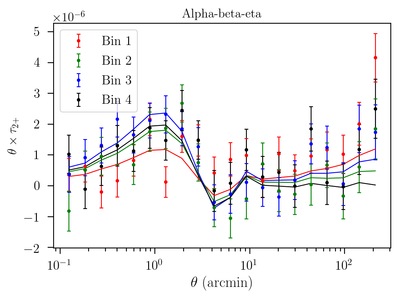
The figure below show one particular set of Tau statistics, for all the tomograpic bins in DES Y3, and in as continues line the best fit model.

PSF error propagation in cosmological estimates

Once we have estimates for $\alpha$, $\beta$, and $\eta$, we can study their effects on the final cosmological estimates using the Rho statistics as follows:

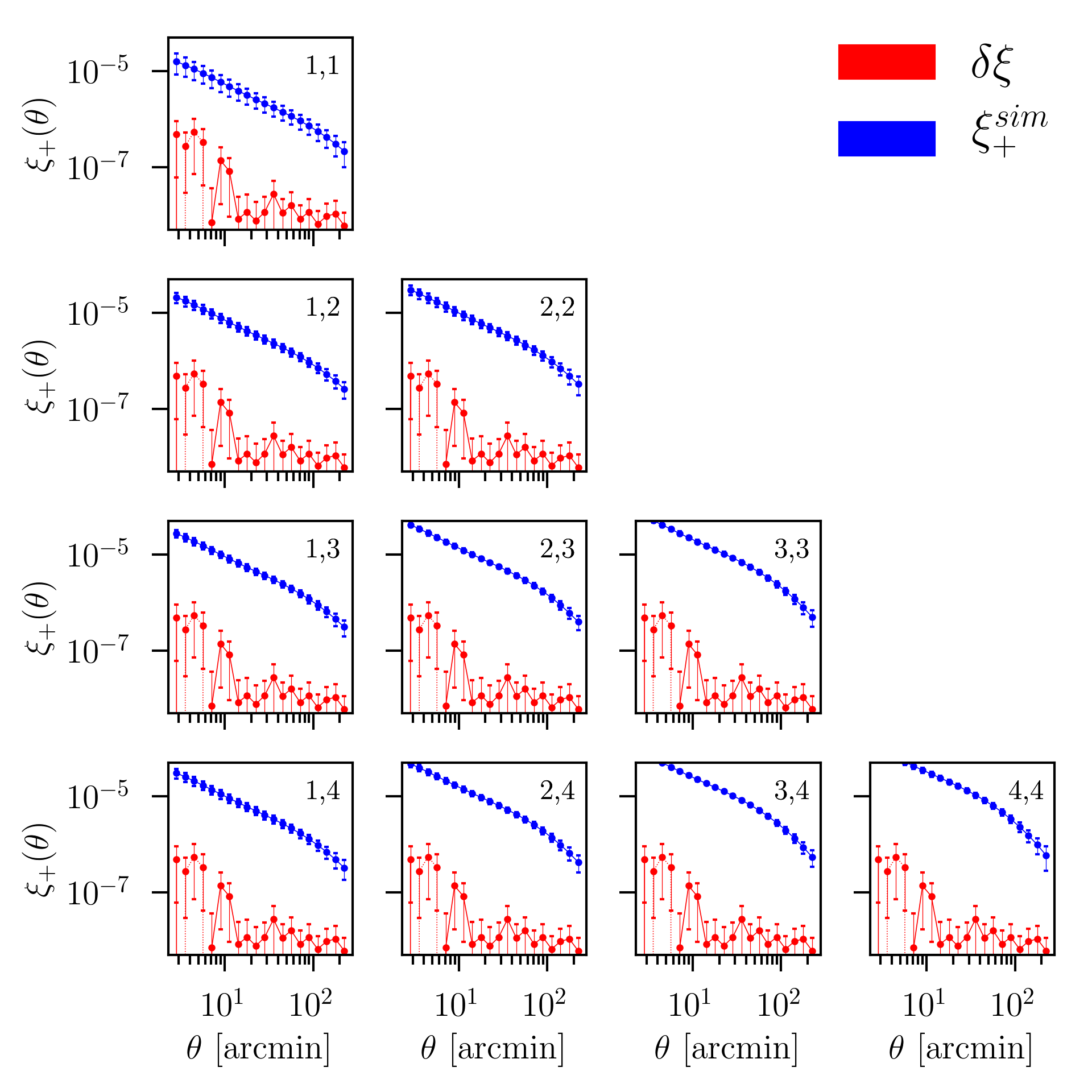
\[\begin{equation} \xi_{+}^{ij'(\textrm{obs})} = \left\langle e^{i'}_{\textrm{obs}}e^{j'}_{\textrm{obs}} \right\rangle = \left\langle ( \gamma^{i'} + \delta e^{i'}_{\textrm{sys}}) ( \gamma^{j'} + \delta e^{j'}_{\textrm{sys}} )\right\rangle \end{equation}\] \[\begin{equation} \xi_{+}^{ij'(\textrm{obs})} = \xi_{+}^{'(t)} + \left\langle \delta e^{i'}_{\textrm{sys}}\delta e^{j'}_{\textrm{sys}} \right\rangle , \label{eq:sheartwopointtomocontamination} \end{equation}\] \[\begin{equation} \xi_{+\textrm{obs}}^{ij'}= \xi_{+ t}^{ij'} +\left\langle (\alpha^{i} e^{p'}+ \beta^{i} q'+\eta^{i} w')(\alpha^{j} e^{p'}+ \beta^{j}q' +\eta^{j} w') \right\rangle \end{equation}\] \[\begin{equation} \boxed{ \begin{aligned} \xi_{\textrm{obs}}^{ij'} =\xi_{+ t}^{ij'} +\alpha^{i}\alpha^{j} \rho_{0}+ \beta^{i}\beta^{j} \rho_{1} + \eta^{i}\eta^{j}\rho_{3} + \left(\beta^{i}\alpha^{j} + \beta^{j}\alpha^{i}\right)\rho_{2}+ \\ \left( \alpha^{i}\eta^{j}+\alpha^{j}\eta^{i} \right)\rho_{5}+ \left(\beta^{i}\eta^{j}+\beta^{j}\eta^{i} \right)\rho_{4}. \end{aligned} } \label{eq:tomographicbias} \end{equation}\]

We now have the shear 2PCF contamination due to PSF additive systematic biases $\delta \xi$, as a function of Rho statistics and the best-fitted $\alpha$, $\beta$, and $\eta$. The figure below shows the comparison of the PSF contamination and the fiducial cosmology data vector. Notice that the contamination is subdominant, almost two orders of magnitude below the fiducial values.

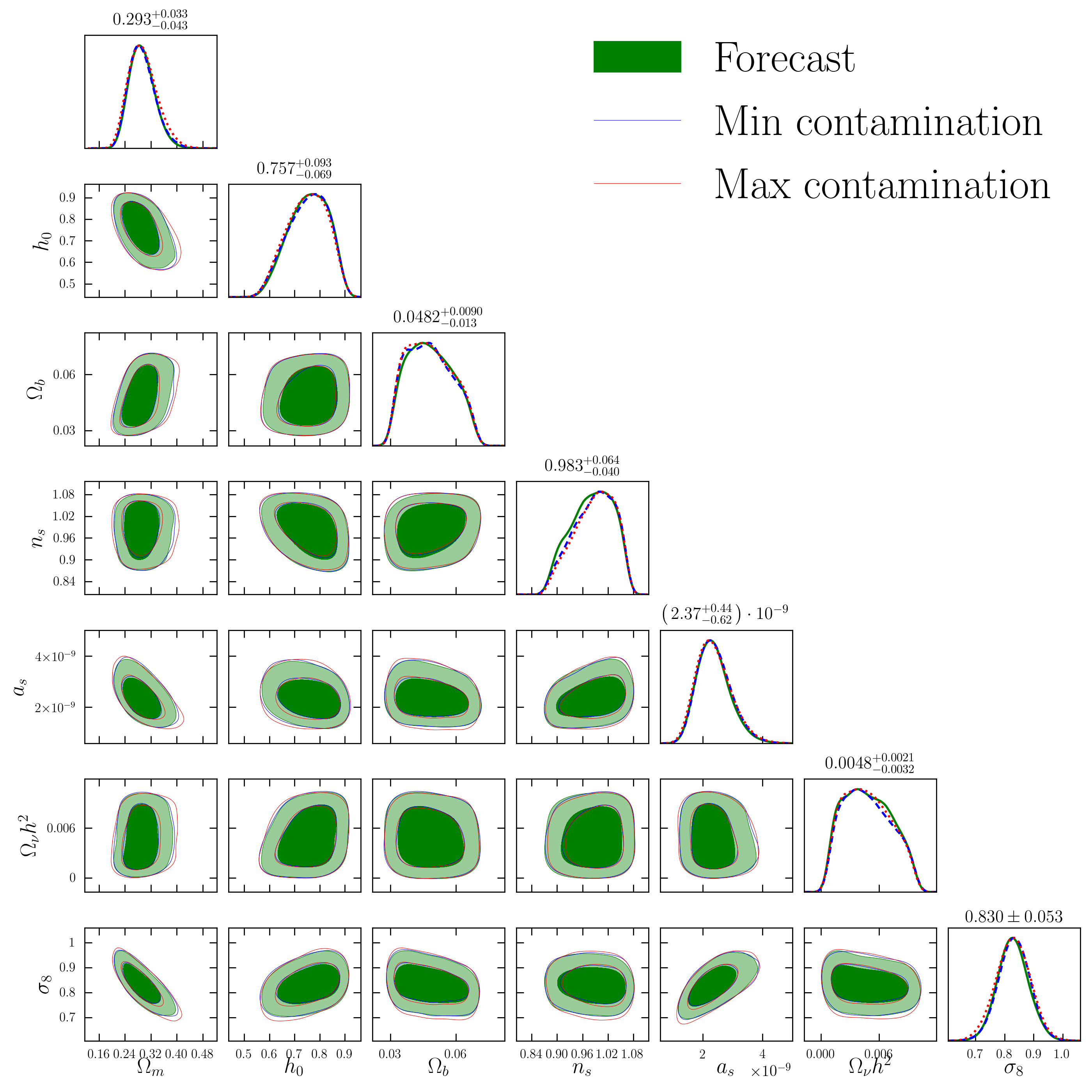
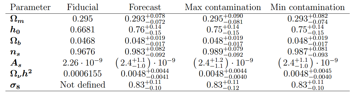
By using the $+1\sigma$ values of the PSF contamination, we can create a test data vector by adding and subtracting it from the fiducial cosmology. With this contaminated data vector, we can perform a likelihood analysis for final cosmological estimates and confirm that this effect is indeed subdominant. The figure below shows the contour plots obtained.